Training robot policies in MuJoCo, and transfer to Webots
Intelligent Systems for Robotics · Week 3
Where we are
Choose a pose, drive there
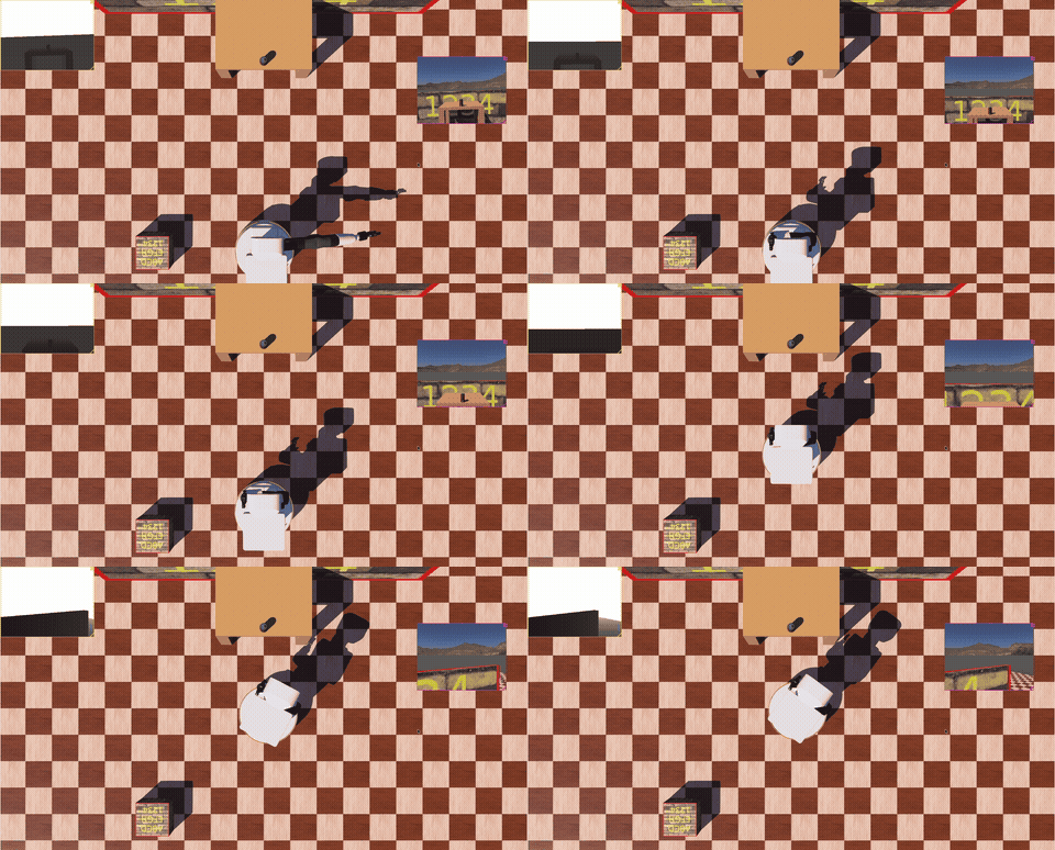
- A sampler chooses where the base should stand to reach the can
drive_todrives there: straight at the point, then a turn in place
Start A, twice real time. It stopped 19 cm from the pose. PYTHONPATH=. python3 examples/03-training-policies/main.py --webots
Where the base stopped
| Start | Proposed pose | Reached, by odometry | Off by | IK reaches the can? |
|---|---|---|---|---|
| A | x 0.985, y 0.038, yaw 0.212 | x 0.978, y 0.038, yaw 0.125 | 0.7 cm, 5.0° | yes |
| B | x 1.006, y −0.344, yaw 0.920 | x 1.030, y −0.308, yaw 1.007 | 4.3 cm, 5.0° | yes |
| C | x 0.927, y 0.347, yaw −0.608 | x 0.993, y 0.193, yaw −0.693 | 16.7 cm, 4.9° | no |
The heading is right to 5°. The position is under 1 cm out from A and 17 cm out from C, where the arm no longer reaches the can. The base slides during the final turn in place.
Does learning beat drive_to here?
| Start A | Start B | Start C | |
|---|---|---|---|
drive_to alone |
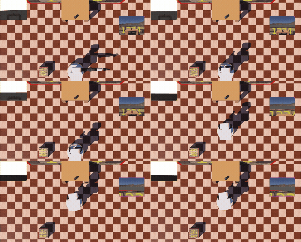 0.7 cm off, 6 s |
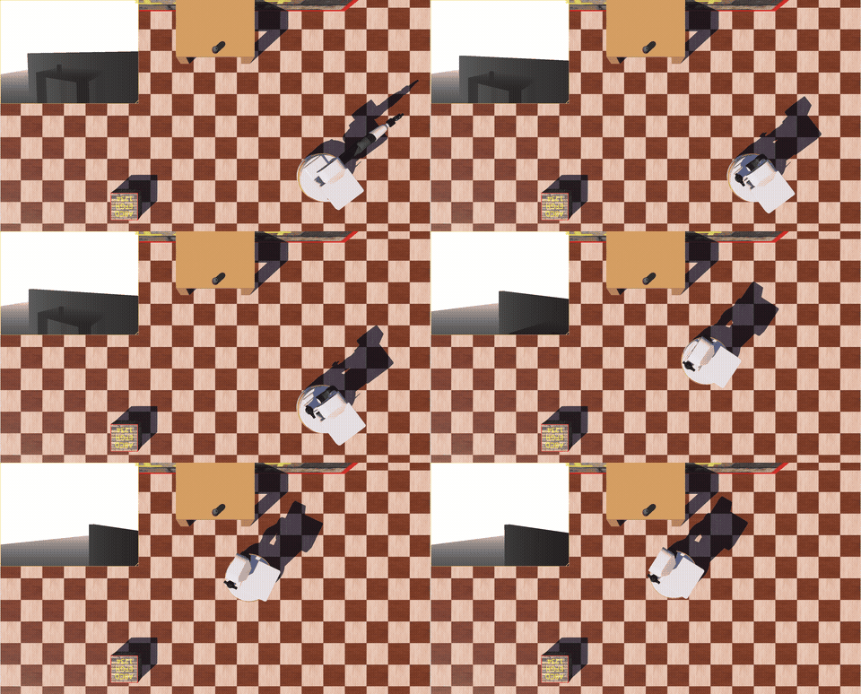 4.3 cm off, 8 s |
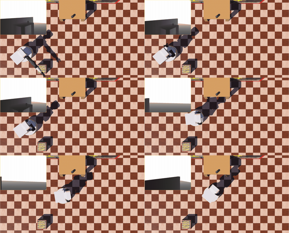 16.7 cm off, the arm cannot reach |
| Docking policy | 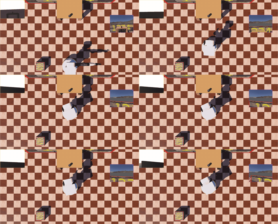 3.7 cm off, timed out at 30 s |
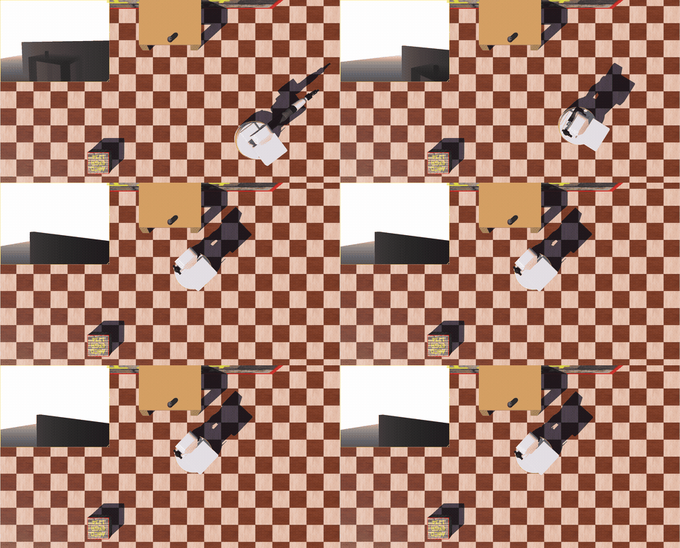 1.1 cm off, 27 s |
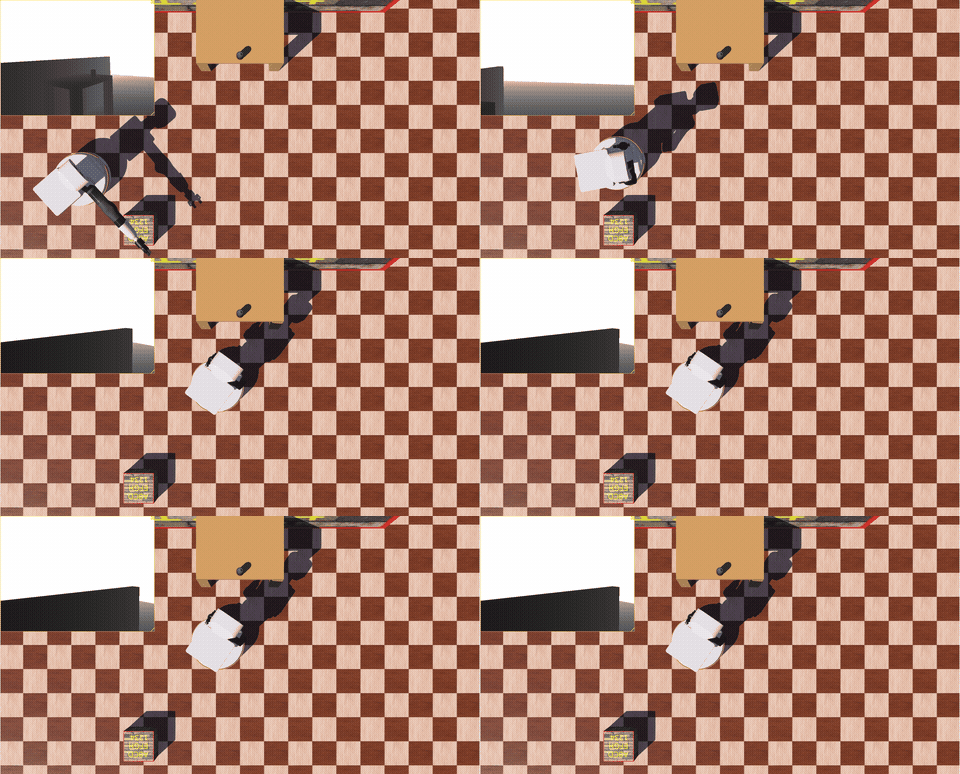 6.8 cm off, timed out at 30 s |
From A, drive_to wins. From B and C, the policy does.
Twice real time, by odometry. Run: main.py webots-placement --start A, or webots-chain.
The last metre, against a real baseline
| Dock controller | From anywhere | Lined up |
|---|---|---|
| Learned docking | 71% | 82% |
| Pose controller | 42% | 60% |
drive_to's control law | 14% | 78% |
goto_empty.zip | 35% | 52% |
Every controller steers on the same goal, anchored to the table's legs.
From anywhere, the policy leads by 29 points. Lined up, by 5, at the edge of the noise.
Both rivals turn in place. A rival that follows an arc, as TIAGo should drive, is not measured yet.
Which of these should have been learned?
- Where to stand
- How to drive the last metre
- How to get across a room with furniture in it
Today answers each one with a measurement.
Today
- Designing an environment: state, reward, termination
- Placement: a learned policy against a sampler
- Transfer: what a second simulator finds
- Obstacles, still open
- Your micro-project
Part 1
An environment is a design
Week 2 took the environment as given. On a robot, you write it.
- State: what the policy is shown
- Actions: what it can command
- Reward: what it is paid for
- Termination: when an episode ends, and why
- Scenes: what it trains on
The algorithm is the smallest decision on this list.
State: the Markov property
\[ P(s_{t+1} \mid s_t, a_t) = P(s_{t+1} \mid s_0, a_0, \dots, s_t, a_t) \]
The next state depends on the present state and action, and on nothing earlier. Everything the future depends on has to be in \( s_t \).
A policy sees only its observation. What the observation leaves out, no amount of training can recover.
CartPole without velocity
Show the policy only the cart position \( x \) and the pole angle \( \theta \).
- A pole at 5° falling right
- A pole at 5° swinging back up
Same observation, opposite correct actions.
Fix it by adding \( \dot{x} \) and \( \dot{\theta} \), or by stacking the last two observations so the policy can difference them.
State: choose the frame
Goal in the world frame
\( (x_g, y_g) = (3.0, 2.0) \)
Means nothing without the robot's own pose. The policy has to learn the transform.
Goal in the robot frame
\( (\Delta x, \Delta y) = (1.2, -0.4) \)
"Ahead and to the right." The same situation anywhere in the room gives the same input.
A frame that makes equivalent situations look the same is data the policy does not have to collect.
State: only what the robot can know
The simulator will hand you anything:
- the robot's exact pose
- the table's exact box
- contact forces, every object's velocity
The robot in Webots has a lidar, odometry and a detector. Your
observe runs there too, unchanged.
If observe reads it, the robot must be able to measure it.
State: noise and scale
- Trained on exact inputs, a policy relies on a precision it will not have. The homework's training adds 2 cm of noise to the object and 1 cm to each range.
-
A scan holds
infwherever nothing returned. A network cannot takeinf. - Inputs of very different sizes, metres next to radians next to counts, slow learning. Bring them to comparable ranges.
Actions: given this week
The action space fixes what a policy can express at all.
- Placement: three numbers in \( [-1, 1] \) that become a pose around the can. Slide 29.
- Docking: linear and angular velocity, fixed by the policy you start from.
You will see that a good action space can do most of the work.
Reward: sparse or shaped
Sparse
1 on success, 0 otherwise.
Says exactly what you want. Gives no signal until the first success.
Shaped
Extra terms that pay for progress.
Learns faster. Also changes what is optimal, unless you are careful.
Shaping gone wrong
A simulated bicycle was paid for progress towards its goal, and was not penalised for moving away.
It learned to ride in tiny circles near the start.
Each circle contains a stretch towards the goal. That stretch pays, and the rest of the circle costs nothing.
Randløv & Alstrøm (1998), reported in Ng, Harada & Russell (1999).
Potential-based shaping
Pick any function of state, \( \Phi(s) \). Add
\[ F(s, s') = \gamma \, \Phi(s') - \Phi(s) \]
to every reward. The optimal policy does not change.
Example: \( \Phi(s) = -\,d(s, \text{goal}) \). Moving closer pays, moving away costs the same amount back.
Ng, Harada & Russell (1999), ICML, 278–287.
Why a loop earns nothing
With \( \gamma = 1 \), round a loop that returns to \( s_0 \):
\[ \sum_{t=0}^{T-1} \bigl( \Phi(s_{t+1}) - \Phi(s_t) \bigr) = \Phi(s_T) - \Phi(s_0) = 0 \]
The sum telescopes. The bicycle's circles are worth exactly nothing.
Any term that is not of this form is a new task. Check what that task rewards.
What does this reward make optimal?
Every term in a reward is a price. The agent pays whatever is cheapest.
The question to ask of a reward is what it makes optimal. What you hoped it would encourage is a different question.
A boat race
CoastRunners pays points for hitting targets along the course. An agent trained on the score found a lagoon where targets respawn.
It circled there, crashing and catching fire, and never finished the race. It scored 20% higher than human players.
Clark & Amodei (2016), "Faulty reward functions in the wild", OpenAI.
A vacuum cleaner
Pay a vacuum robot for the amount of dirt it picks up.
It can pick up dirt, dump it, and pick it up again.
Russell and Norvig's rule: measure what you want in the environment, a clean floor, and not how you think the agent should behave.
Russell & Norvig, Artificial Intelligence: A Modern Approach, 3rd and 4th eds., Section 2.2.
Your turn
A pick-and-place arm gets +10 when the cube is in the box, and −1 on every step its gripper touches the table.
The cube sits close to the table's surface, and grasps fail often.
What does this reward make optimal?
Termination and truncation
-
terminated: the task itself ended. Success, a collision. Nothing follows, so no future value. -
truncated: you stopped the clock. The world would have gone on, so the value of the last state still counts.
Gymnasium returns both from step. Confuse them and the value estimates are wrong near the limit.
So running out of time is not an ending. A policy that stops trying pays its cost per step \( c \) for as long as the bootstrap looks ahead: about \( c / (1 - \gamma) \), whatever the limit.
Pardo et al. (2018), "Time Limits in Reinforcement Learning", ICML.
Curricula: start easy
A task so hard that success never happens gives a sparse reward nothing to learn from.
| Docking, 5 cm and 5°, next to a table | Success |
|---|---|
| PPO from scratch, 40 minutes | 0% |
| A policy trained on an empty floor, before any fine-tune | 39% |
Train the easy task first, then fine-tune on the hard one.
Bengio et al. (2009), "Curriculum learning", ICML.
Scenes are part of the design
- What varies from episode to episode: layout, walls, clutter, start pose
- How far, how cluttered, how noisy
- Evaluate on scenes the policy never trained on, with fixed seeds
The same seeds for two designs, or for a design and a baseline, make the comparison fair.
A checklist before you train
- Does the observation hold everything the next step depends on?
- Can the robot measure every input in Webots?
- What does the reward make optimal, including every way to fail?
- Which endings are terminal, and which are the clock?
- What scenes does it train on, and what does it meet later?
Part 2
Placement as a problem
Where should the base stand, so that the arm can reach the can?
- One decision per episode: scan once, propose a pose, done
- Scored by inverse kinematics from that pose: reachable or not
- The base must not collide with the table, a wall or the clutter
The action is object-relative
Three numbers in \( [-1, 1] \): distance, bearing, heading error. Every pose it can express faces the can.
The classical baseline
- Draw an action at random
- Check the pose with inverse kinematics, about 14 ms
- Keep the first one that reaches the can
100% of scenes, a median of 4 samples and 13 ms per decision.
The same object-relative action, searched instead of learned.
The learned policy
| Placement, 200 fresh scenes | Success | 0 walls | 1 wall | 2 walls |
|---|---|---|---|---|
| Naive design, seed 0 | 80.5% (74.5–85.4) | 78.2% | 85.5% | 75.7% |
| Naive design, seed 1 | 80.5% (74.5–85.4) | 79.3% | 84.2% | 75.7% |
| Instructor's design | 89.0% (83.9–92.6) | 92.0% | 86.8% | 86.5% |
| Sampler | 100% |
The naive design sees only the can's position and is paid 1 for success. The instructor's design solves 8.5 points more. The intervals still overlap.
Why so close?
The action does most of the work.
It already restricts every pose to 0.3 to 1.2 m from the can, facing it. What is left is which side to approach from, and a sensible distance.
The walls are where the lidar should help. With two walls it scores 86.5%, against 76% for both seeds of the naive design, on 37 scenes. Without walls it also leads, 92% against 78 and 79%.
What learning buys here
- A forward pass of the network: under 1 ms
- The sampler: one or more IK solves at about 14 ms each
Training is paid once. Every later query is cheap. The policy is the sampler's search, amortised.
It matters only where placement is queried many times.
Success is not the only cost
| Placement | Success, of 200 | Distance, median (IQR) | Turning, median | Stand-off, median | Within 10 cm of an obstacle | Time per decision |
|---|---|---|---|---|---|---|
| Naive design, seed 0 | 161 | 0.86 m (0.53–1.25) | 64° | 0.98 m | 9 | under 1 ms |
| Naive design, seed 1 | 161 | 0.88 m (0.55–1.23) | 70° | 0.99 m | 10 | under 1 ms |
| Instructor's design | 178 | 1.34 m (0.85–1.82) | 77° | 0.79 m | 1 | under 1 ms |
| Sampler, first accepted | 200 | 1.60 m (1.06–2.26) | 129° | 0.82 m | 21 | 9 ms |
| Sampler, nearest of 64 accepted | 200 | 1.01 m (0.69–1.39) | 46° | 0.90 m | 28 | 230 ms |
On the 127 scenes all of them solved. Paid 1 for success, the policy stands at the edge of the arm's reach, 0.98 m from the can. The instructor's design stands 0.79 m off and keeps 10 cm clear, and drives further to do it.
Closer still: learned only, or then slide in?
| Placement, instructor's design | Learned only | Learned, then slide_in |
|---|---|---|
| Solved, of 200 | 178 | 172 |
| Stand-off, median | 0.79 m | 0.75 m |
| IK still reaches after a 5 cm, 3° arrival error | 87% | 85% |
| Time per decision | under 1 ms | 47 ms |
slide_in keeps the policy's bearing and heading, and moves the base in
to the nearest stand-off IK accepts with 10 cm clear, keeping 10 cm in hand.
4 cm closer, for 47 ms a decision. Part 1 leaves the choice to you.
Use both: learn the order, keep the check
- The sampler draws 64 candidate poses
- A classifier trained on IK verdicts scores each one's chance of success
- IK checks them best first. If none passes, 64 random ones follow.
| Order | Solved, of 200 | First candidate accepted | IK calls, median | Time, median |
|---|---|---|---|---|
| Random | 197 | 39–46 | 3 | 11–21 ms |
| Learned ranking | 198 | 151–163 | 1 | 2 ms |
The sampler's success in 2 ms instead of 11 to 21. Learning becomes a heuristic inside the classical method.
Action-related places
- Run many simulated grasps from base poses around an object
- Learn the probability that a grasp succeeds from each pose, relative to the object
- At query time, sample where the object might be, and pick the pose most likely to succeed over all of them
Least commitment: the robot keeps a region of good places, not one pose.
Stulp, Fedrizzi, Mösenlechner & Beetz (2012), JAIR 43, 1–42.
The same quantity, twice
Placement is one step, rewarded 1 for success and 0 otherwise. So
\[ Q(s, a) = \mathbb{E}[\, r \mid s, a \,] = P(\text{success} \mid s, a) \]
SAC's critic estimates what an action-related place represents. Its actor learns to output the best action directly, where Stulp et al. search.
This reading is the course's. The paper states that an action-related place is not a reinforcement learning policy.
Their baseline, and ours
- Stulp et al. compare against a fixed offset from the object
- Ours checks every candidate with inverse kinematics before accepting it
Against a sampler with an IK check, a learned placement can only win on time.
Part 3
Transfer: what a second simulator finds
Train in MuJoCo. Run the same code on Webots' TIAGo.
Two simulators disagree in ways a real robot would too. They also disagree where one of them, or your code, is wrong.
Bug 1: the lidar was mirrored
- A box on the floor to the robot's left read at −94°, on its right
- Webots orders the range image left to right. The bridge's header said right to left.
- Every test passed. Both backends agreed with the wrong header.
A policy trained on one side of the world would have met the mirror image.
Bug 2: the robot sees itself
- In Webots, 52 beams hit TIAGo's own body at 0.23–0.27 m, at ±108–117°
- MuJoCo's scan never does
- Returns under 0.3 m now read as no return, but only beyond ±100°
The first mask applied at every angle. In 66% of one policy's collisions, the obstacle was the return the mask had thrown away.
Bug 3: the arm was out
| Start | Arm as loaded | Arm tucked |
|---|---|---|
| A | 19.4 cm, 59°, timed out | 18.1 cm, 4.6° |
| B | 25.5 cm, 60°, timed out | 15.4 cm, 4.9° |
| C | 3.4 cm, 4.5° | 22.8 cm, 4.4° |
Training assumed the arm tucked. In Webots it was not, and the palm met the table during the final turn.
The casters, from week 1
TIAGo has four passive casters. After a spin in place they trail sideways, and the next straight leg drags.
| Week 1's square | Closure, odometry | Ground truth |
|---|---|---|
| Spin in place, hold heading | 0.418 m | 1.443 m |
| Turn as an arc, hold heading | 0.084 m | 0.174 m |
Webots turns half as far as asked
- Commanded 160° in place, arm tucked: reached 72–78°
- The wheels reach half the commanded speed. The motors' 10 N m saturate against the casters.
- MuJoCo as vendored, same limits: 142°
A policy trained on 142° would turn twice as far as it meant to, then correct forever.
Calibrated by load
- Caster damping up to 100 times, and friction doubled: the spin stayed above 114°
- Lowering MuJoCo's casters by 0.4 mm moves weight onto them: 68–76°
- 0.75 mm gives 58–64°. At 1 mm the drive wheels lift off the floor.
Drift after the turn: 35.4° mean in MuJoCo, 33–40° in Webots.
Randomise what you cannot pin down
Every training episode draws its own caster drop, 0.25–0.55 mm, and damping, half to twice nominal.
That spans spins of about 55–90°. Webots is one draw among many.
Tobin et al. (2017), IROS, randomised appearance. Peng et al. (2018), ICRA, randomised dynamics.
Train on the truth, deploy on a landmark
- Odometry drifts. The goal is re-anchored every step to the table, fitted to its legs in the lidar scan.
- In Webots, 60 of 60 scans fitted, median error 4–11 mm
- Trained on the exact pose, the same policy scores 68.5% on the exact pose and 69% on odometry and the landmark
The landmark is close enough to the truth that the policy need not learn its noise.
What transferred
- Placement: IK reached the can after every Webots trial, with no code change
- Docking: ran unchanged; three starts cannot rank it against a classical dock
- Three bugs no unit test could have found
Each bug was found by running the same code on a second simulator.
Part 4
Obstacles, still open
go-to | Training | Success |
|---|---|---|
| PPO, empty floor, from scratch | 10 minutes | 100% of 200 |
| The empty-floor policy, among obstacles | none | 42.5% |
| PPO, obstacles, from the empty-floor policy | 27 minutes | 46.5% |
| SAC, obstacles, from scratch | 1 hour | 10% |
Minutes on an empty floor. Among furniture, training barely moves it.
What did not fix it
- The self-hit mask, corrected
- Starts kept 0.8 m clear of obstacles: the base turns on arcs of about 0.7 m
- A penalty for passing close to obstacles
- The simulator's exact pose instead of odometry
- SAC instead of PPO
- Another reward, from the empty-floor policy or from scratch
- A depth camera on the head
- Progress measured along the free path, not the straight line
Each changed the result by less than the noise, or not for long. All tried before the simulator fix.
It sees the obstacle and does not go round
| Straight line to the goal | Scenes | Success |
|---|---|---|
| Clear | 99 | 90% |
| Blocked | 101 | 5% |
72% of its collisions are inside the lidar's view, where the route round was a median 1.10 m wide, for a base 0.54 m wide.
The course's answer: perception names the obstacle, the world model records it, and a graph search plans the route. Learning keeps the last metre.
Slide 7, answered
| Problem | Learned? | Why |
|---|---|---|
| Where to stand | Optional | A sampler succeeds; learning makes it fast |
| The last metre | From anywhere | Lined up, a classical controller on the table's legs comes within 5 points. No arc-path rival yet. |
| Across a room | Not yet | Planned over the world model instead |
Learn what classical methods do badly.
Part 5
Your micro-project
Placement
- Design the observation and the reward
- 200 scenes, against both samplers
- Webots from A, B and C
Docking
- Design the reward, fine-tune
- Before and after, and
tolerance - Webots chain from A, B and C
- Price every ending
In exercises/03-training-policies/, results in RESULTS.md.
The training loops are provided
train-placement
- SAC, replay buffer, batches of 256
- 200 000 steps by default
- 2 cm noise on the can, 1 cm per range
train-docking
- PPO, continuing from
goto_empty.zip - 12 288 steps per update, whatever the workers
- Learning rate 1e-4, a third of the stored 3e-4
- 1.8 million steps: 35 minutes on 4 workers
The notes page explains both, step by step. Start train-placement first; it runs while you read.
Done when
eval-dockinggives 39.0% forgoto_empty.zip. If not, check your seeding first.- Your docking policy succeeds at least 10 points above that, on the same 200 episodes. That shows the fine-tune ran.
- Every table in
RESULTS.mdis filled; the Webots rows have no threshold - Your docking paragraph prices every ending and names the cheapest
These are targets for checking your own work, not pass marks. The README's Self Check has the full list.
Reading
- Poole & Mackworth (2023), Artificial Intelligence, 3rd ed., Cambridge University Press. Sections 13.1 and 13.9
- Stulp, Fedrizzi, Mösenlechner & Beetz (2012), JAIR 43, 1–42. Sections 1, 3.1, 4.1 and 6.2
- Ng, Harada & Russell (1999), Policy invariance under reward transformations, ICML, 278–287